Add Oil fluctutations to the simple RBC Model in Stata
In this modified version of the simple RBC model, we've introduced a significant enhancement by incorporating oil price fluctuations. Traditionally, the RBC model focuses on the role of technology shocks in driving economic cycles. However, in today's complex global economy, oil prices have a profound impact on economic stability. To address this, we've integrated oil as a fundamental input into the model's production process. Now, not only do firms rely on capital and labor, but they also depend on oil to produce goods. What distinguishes our model is its streamlined approach to representing oil supply dynamics. We simplify the analysis with an exogenous representation of oil supply, which indeed implies how oil supply is unpredictable. This modification allows users to explore how oil shocks influence economic outcomes, making it a valuable tool for understanding and analyzing the modern economic landscape."
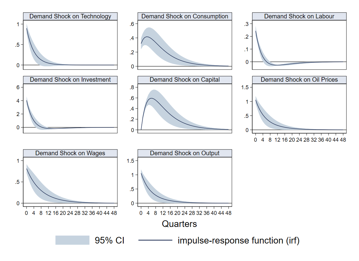
Demand Shock
In this simple RBC model with exogenous oil supply, we have identified two shocks: Demand Shock and Supply Shocks. A demand shock is characterized by an increase in firm productivity, leading to greater input demand for output production. As the demand for oil input rises, we observe a corresponding increase in oil prices—a straightforward application of the law of supply and demand.
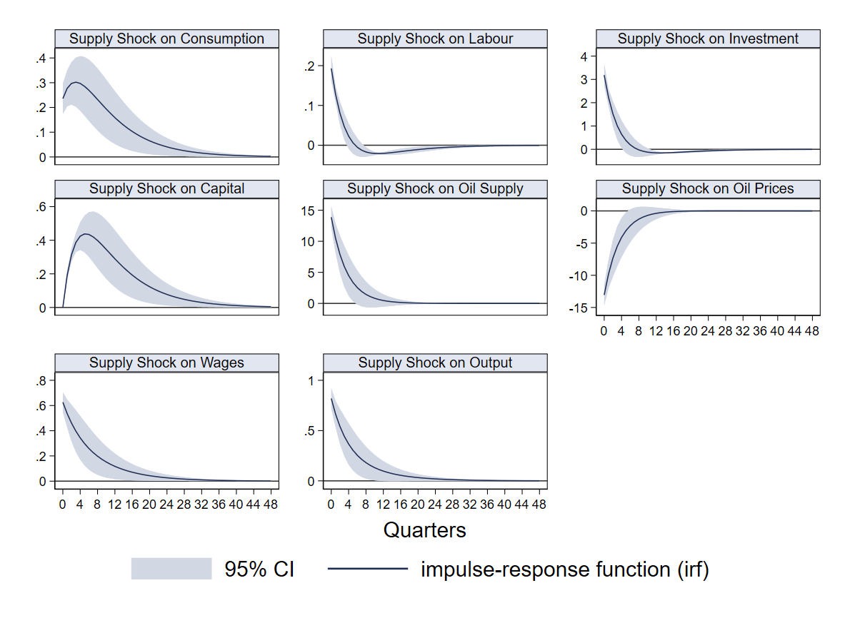
Supply Shock
A supply shock is characterized by an increase in the productivity of oil suppliers, resulting in higher oil production. As the supply of oil increases, we observe a corresponding decrease in oil prices—a straightforward application of the law of supply and demand.
RBC Model with Oil Production - STATA
On Sale
$10.00
$10.00
The package includes:
- Dataset
- Complete DO file
- PDF with Math Solution
Also, the PDF includes some ideas to improve the model and improve your skills.
Please Note: The model is the same I taught in my course DSGE models in Matlab Dynare. This package is the adaptation of the model to STATA.
Important Information
The oil model is the same as that in my DSGE models in the Matlab with Dynare course. This is just the corresponding code to replicate the model in STATA. If you've already purchased the Matlab course, your knowledge should enable you to reproduce it in Stata as well. However, it can still be highly beneficial to acquire this package, especially if you're interested in having access to all the specific codes or if you encounter difficulties with coding on your own. An important aspect to note is that the model in this package is not pre-calibrated; instead, it's estimated using US Real GDP and Crude oil Prices per barrel in USD.
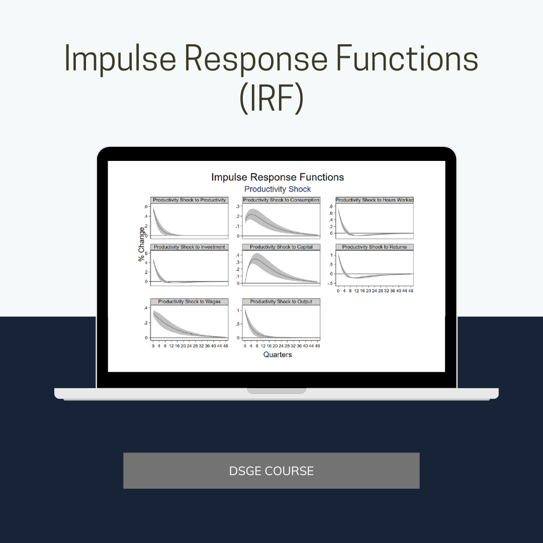
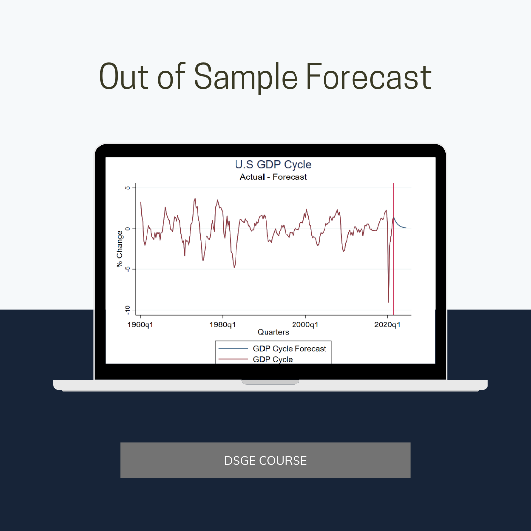
The material includes a comprehensive DO file with codes for generating out-of-sample forecasts, supply shock impulse response functions (IRF), demand shock IRF, and one-step-ahead predictions for capital and output. It comprises a highly intricate and comprehensive code that you won't want to miss out on.
Some of the graphics you will be able to produce....
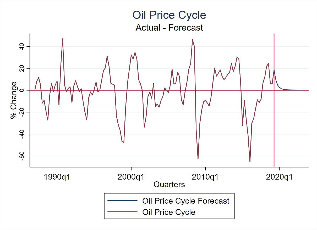
Forecast Oil Prices
The DO file includes the code to replicate an out of sample forecast for oil prices.
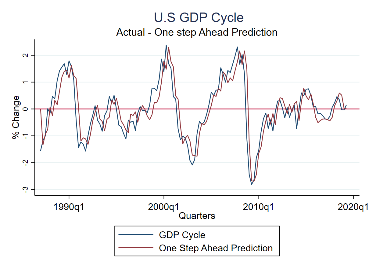
Produce one-step-ahead predictions
The DO File includes the necessary codes to produce one step ahead predictions for the GDP Cycle.
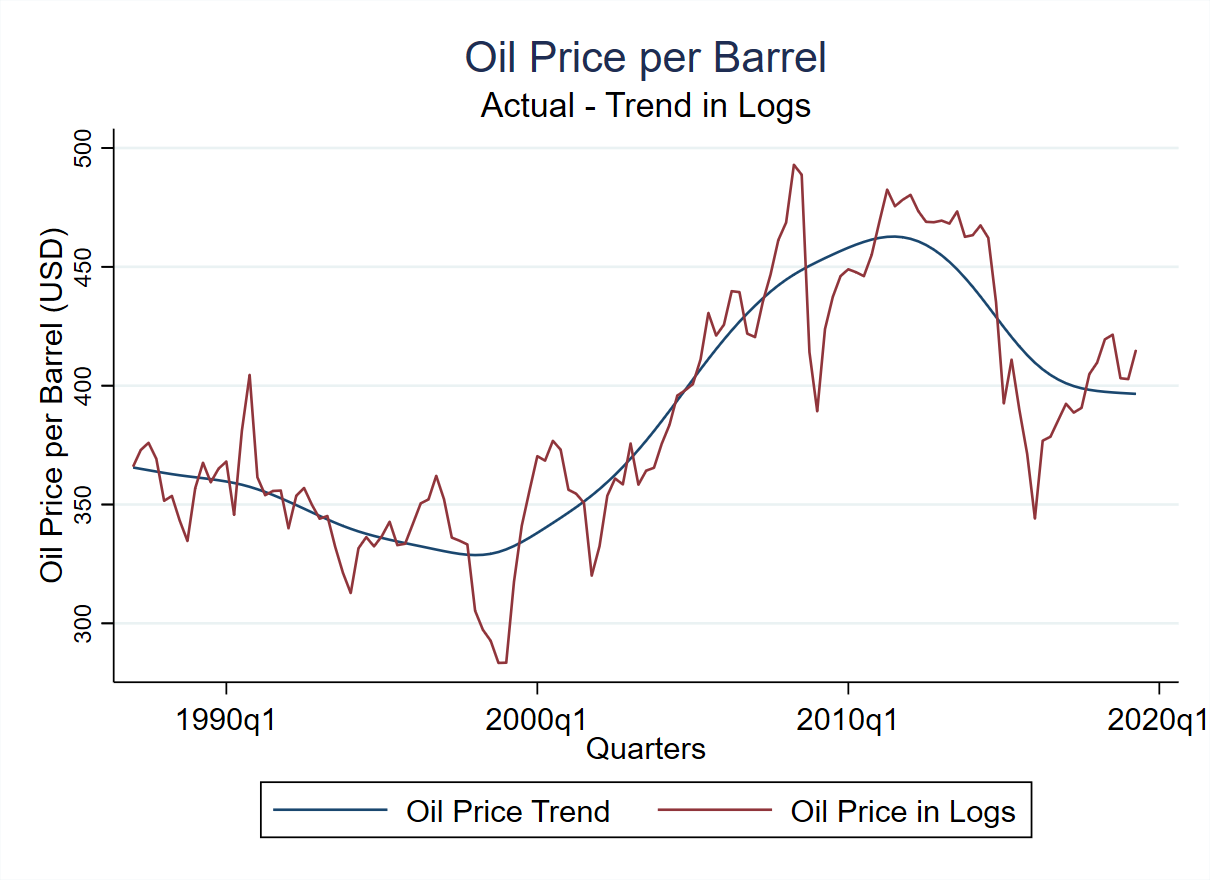
Detrend Series
Use the HP-Filter to decompose a series into trend and cycle. In this, we can see the price of oil per barrel (in USD) in logarithms, and in blue, the trend
RBC model with Oil Production is an extension of the following model:
Make sure to buy the following package (if you haven't yet).


DSGE Course in STATA- RBC Model
On Sale
$14.99
$14.99
Preview
The Dynamic stochastic general equilibrium (DSGE)comprehensive course will teach you how to estimate DSGE models in STATA. The course is designed so that you can learn step by step and get a clear understanding of the concepts. The course covers important topics such as model estimation, forecasting, and policy analysis.